``

Hello and welcome to week 12 of ESPM 112L-

Metagenomic Data Analysis Lab!

• First step: Making your alignment
  • Interlude: .sam files, .bam files, samtools, oh my!
• Geneious
  • Interlude: Predicting ORFs (make sure to do this before continuing!)
  • Back to mapping
• Turn-in assignment

This week we’re going to generate an alignment like you did last week, but we’re going to visualize that alignment in geneious so you can see two things:

1. What coverage actually looks like and what it means
2. SNP-level microdiversity in a population genome

Let’s get to it!

First step: Making your alignment

This week, making your alignment is going to be a bit easier than last week, since we’re going to use a different aligner, called bbmap.sh. Don’t worry- even though it’s a different tool, it’s actually much easier to use, and it will generate your alignment much faster!

First, make a folder in your home directory (call it Lab11 or whatever you’d prefer.) Then, as we did last week, copy in a bin of your choice (from your sample!) to this directory.

Remember to make sure the genome you choose is of generally good quality- at least 1.5Mbp, and the fewer contigs the better!

And, as with last week, we’re going to make symbolic links to your reads into this folder to make them easier to access. Trust me- this saves a lot of typing time and hard drive space.

First choose a bin from your cow, located in /class_data/assemblies/cow_bins

mkdir ~/Lab11

# REMEMBER NOT TO JUST COPY PASTE!
cp /class_data/assemblies/[YOUR COW]/[bin contigs file].fna ~/Lab11

#Go to that directory
cd ~/Lab11

#Make symbolic links to reads
#This takes the QC'd read files and makes links to them in your directory
#So you don't have to write out the full path when you make your command.
ln -s /class_data/reads/[SAMPLE NAME]/raw.d/*trim_clean.PE.*.fastq.gz .

Awesome- now that you’ve done that, let’s go ahead and run your alignment. You don’t have to generate the index in a separate step like you did last week with bowtie2, so that saves you a step here!

Importantly, make sure to specify threads=4 when you run this; otherwise bbmap.sh will take all the available threads and make it difficult for everyone to run their alignments!

#Remember you're now located in ~/Lab11

bbmap.sh pigz=t unpigz=t ambiguous=random threads=4 ref=[bin contigs file].fna in1=[FORWARD READS FILE].fastq.gz in2=[REVERSE READS FILE].fastq.gz out=stdout.sam | shrinksam | sambam > [genome name].shrink.sort.bam

Just put in values for [bin contigs file], the forward and reverse reads files, and name the final output ([genome name].shrink.sort.bam) what you’d like- I would name it based on the name of the genome you’re looking at. Say we’re using Cow_8_31_maxbin.scaffolds2bin.tsv_bin_126.fa; in that case I would name the final output Cow_8_31_maxbin.scaffolds2bin.tsv_bin_126.shrink.sort.bam or something similar.

This process should only take a few minutes. bbmap.sh is generally much faster than bowtie2, one of the most commonly used alternatives. Note that this is, of course, dependent on both the size of the genome you’ve chosen and the number of reads in your dataset that you’re aligning to the reference genome.

The additional stuff at the end of the command is various bits of processing; filtering, sorting, and shrinking your alignment file by removing uninformative bits. Let’s talk for a bit about what’s happening there.

Interlude: .sam files, .bam files, samtools, oh my!

There are two kinds of read alignment files, which are generated by read mapping programs like bowtie2 (which you used last week) and bbmap, which you’re using this week.

The first is a .sam file, which stands for Sequence Alignment Map. They look like this:

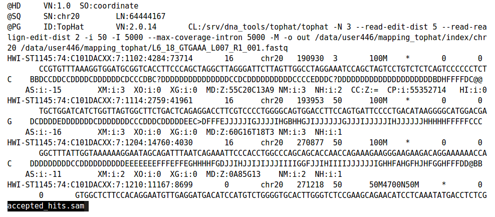
The information here basically is:

• Where on the reference genome your reads align
• How well those reads match your reference

Which is fantastically useful information, as you’ve probably surmised due to our having generated such alignments several times so far in lab. However, there’s a caveat: it’s all in text format! This ends up being very costly in terms of hard drive space (they can each be many gigabytes in size) and computational power (if you have to load a 30GB file every time you do something, it gets old quick).

In order to reduce the amount of space these files take up, we first shrink the file by removing unmapped sequences from the .sam file (with shrinksam), then convert it to a much smaller binary file, called a .bam (with sambam).

A .bam file contains the same information as a .sam file, but in a much smaller package. This is more efficient for programs to load if you want to analyze your data, and more efficient in terms of how much space it’s taking up on your hard drive!

The command as I’ve written it above actually never even writes a .sam file to the hard drive, instead feeding the alignment information directly into programs which will process it and then turn it into a .bam file. If you’re interested in further particulars of how this command works, let me know, and I’ll be happy to explain it to you in greater detail.

Geneious

Now that you’ve finished generating this alignment, let’s download both the alignment (the .bam file) and the bin contigs fasta file you used to generate the alignment to your local PC; we’re going to boot them up in geneious.

Geneious is a versatile platform for doing genomics analysis in a GUI (Graphical User Interface)-based environment. It’s especially great for viewing alignments between reads and reference fasta files to see coverage patterns and SNP microdiversity, both of which we’re going to do today.

If you haven’t already, please download geneious and activate the free trial, which will last 30 days (plenty of time for you to use it for your projects, if you wish). https://www.geneious.com/free-trial/

Before you do anything else, make sure your .bam and .fasta files are both downloaded from the cluster!

Once geneious has been activated, go ahead and boot it up; here’s how to visualize your alignment in geneious.

1. Import your .fasta file first!

Once geneious has started, go up to File -> Import -> From File and select your genome fasta. When you see the pop-up below, say ‘create sequence list’.

1. Now import your .bam file.

Go again to File -> Import -> From File and select your .bam file. Make sure that you’ve clicked on your fasta file to select it before you do so!

Once you’ve got it imported, you’ll see a bunch of scaffold/contig names. Click on one, and let’s see the reads that align to that scaffold. It should look something like this, although all coverage patterns will be different:

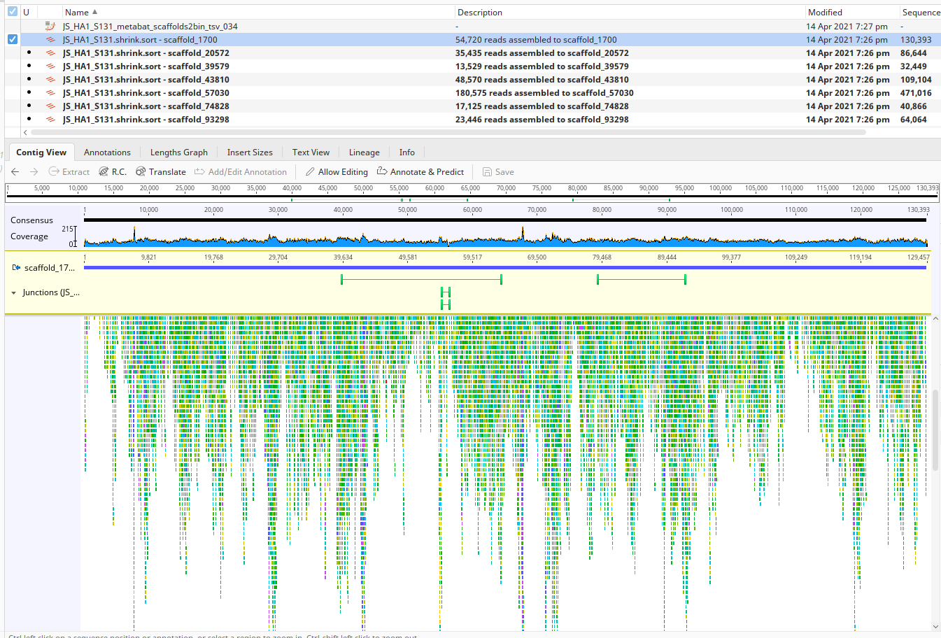
Let’s take a moment to see what’s going on here.

Zoom in (scroll as you would on a browser, or use ctrl + +) and you can see something very different:

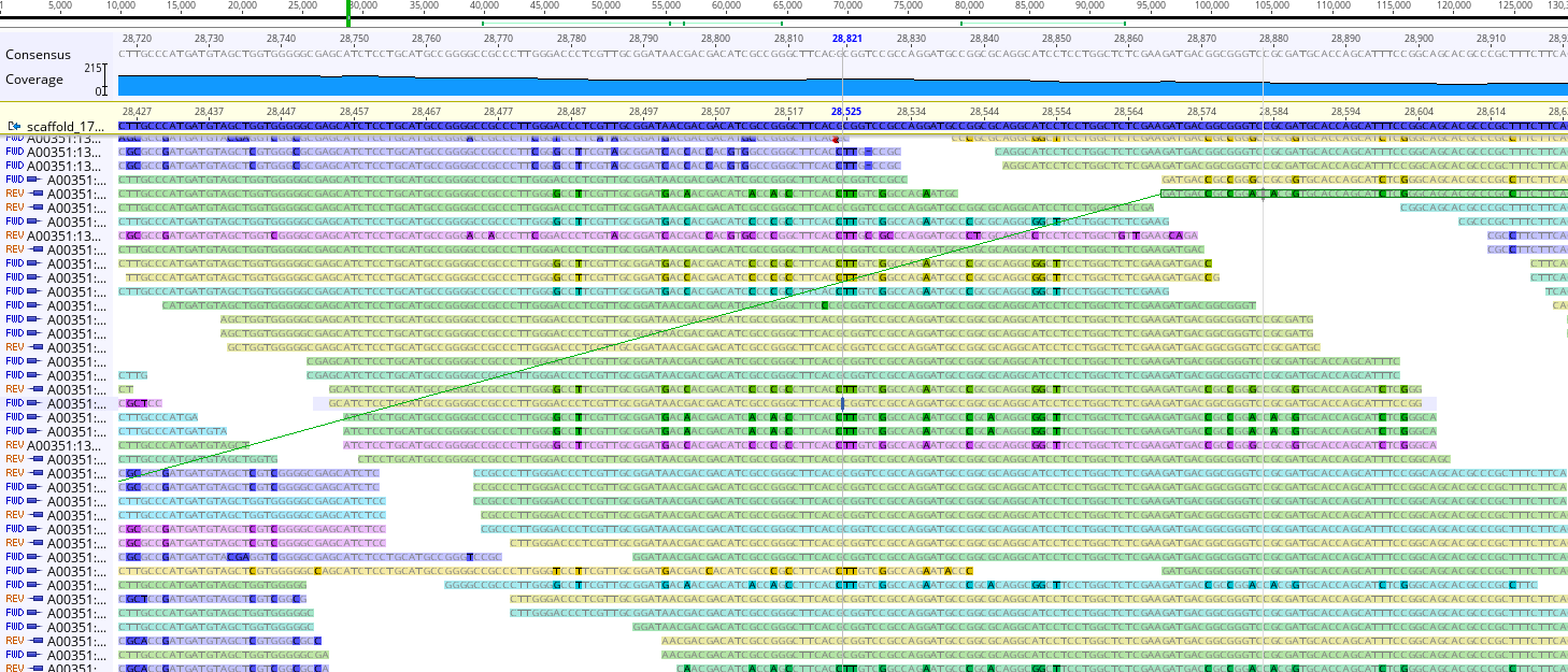
See now how there are highlighted nucleotides? These indicate positions in the reads which disagree with your reference genome. (e.g. Your reference genome says GATTACA and the read might say GATAACA; the fourth nucleotide is different between the two.) These are SNPs; Single Nucleotide Polymorphisms; positions where a single nucleotide mutation has occurred.

Also note that if you roll your cursor over a given read, that read’s mate pair will be highlighted.

1. Make a more stringent mapping

Have you noticed that there’s a ton of mutations around? We generally don’t want to see all of the low-identity reads, since they may really belong to other assembled contigs rather than the one you’re interested in. So let’s go ahead and change that.

First, we want to make separate geneious files for A. the contig of interest, and B. the reads which align to that contig. We’re only re-aligning the reads which already map to this contig, so it’s much easier computationally. You can do it easily on your laptop in probably around a minute!

• Making separate geneious files

First, make sure you’re zoomed in to the point that you can see the names of individual reads (like the below example)

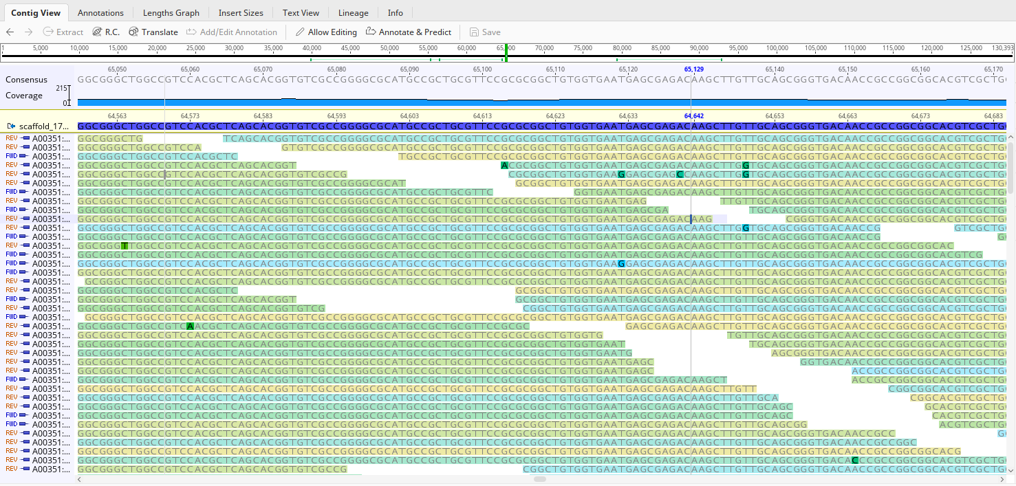
Click on the name of your contig - in my example, it says ‘scaffold_17’ near the top left corner- and then navigate to the ‘extract’ button on the top right. Click on that and choose a name (the default is fine), then press ‘OK’. In your top menu, where you see a bunch of file names, you should now see a file for that scaffold.

Interlude: Predicting ORFs (make sure to do this before continuing!)

It’s very useful to be able to see where the genes are along a contig when visualizing an alignment. In order to predict genes, we’re going to need to install a plugin for geneious (don’t worry, it’s easy). Go to the top menu, select ‘Tools’, then click ‘Plugins’. Scroll down in the resulting menu until you find ‘Glimmer’, then click ‘install’. Go to the bottom of the menu and press ‘OK’!

Now, go to the file for your contig, and select ‘Annotate and Predict’, just above where your sequence is displayed. Click the very bottom option- ‘Predict genes with Glimmer’- and press OK.

Back to mapping

Now that you’ve done that, let’s make a separate file for our reads! Go back to your mapping file - now we want to select just the reads. Click on one of the names of the reads (below the scaffold name, they all say FWD and REV), then press Ctrl+A (PC/linux) or Cmd+A (Mac) to select them all. (If you see the scaffold name and/or anything above highlighted, you can de-select them by holding ctrl (PC/linux) or cmd (mac) and clicking the things you don’t want highlighted) After you’ve done this, click ‘extract’ like you did before, and make a new geneious file for just your reads! (Name it “reads” or something easily identifiable)

• Making a new, more stringent mapping

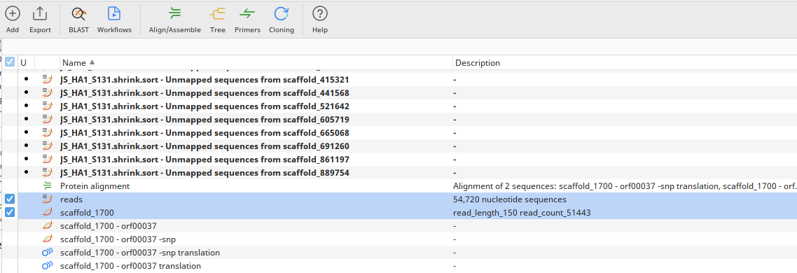
Now select both of these newly created files - the one for just your scaffold and its proteins, and the one for your reads. Go to the top, click ‘Align/Assemble’, and then ‘Map to Reference’.

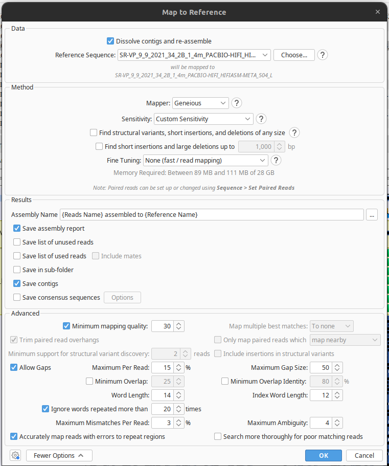
Now, before you do anything else, we want to make sure that this mapping is more stringent, so you can see the difference between a standard mapping and one done with more stringent parameters. In the box that comes up once you’ve clicked ‘Map to Reference’ (see below), there’s a field that says ‘Sensitivity’; click on it and select ‘Custom’. Now, go to the bottom of the box, and click where it says ‘More options’. You should now see all the fields in the below example. Set ‘Maximum mismatches per read’ to 3%, then press OK to begin your new alignment!

Turn-in assignment

1. On the scaffold you’ve re-made the alignment for, what is the maximum coverage value for A. the original mapping, and B. the more stringent mapping?
   • You can find this by looking at your coverage graph and zooming in to the peaks. The legend should also go from 0 to the maximum coverage value to make things easier.

2. Take a screenshot of at least three SNPs that A. occur in more than one read, and B. occur in the coding sequence of a gene.

3. What gene on your contig has the highest coverage? Click on the orange symbol representing that gene, which will show you the amino acid translation, then put that sequence into blastp. What is this gene- does it have any informative annotations?

4. Projects are coming up - submit at least one idea for your group’s project (or individual project, if you prefer) along with today’s turn-in.